The Power of Interdisciplinary Thinking
I’ve always been drawn to the new and different: the ideas that push boundaries, challenge assumptions, and redefine what’s possible. Whether it’s uncovering patterns in data, questioning long-held beliefs in technology, or exploring the social forces that shape our world, I love the process of discovery. I’m drawn to understanding how things work—not just taking them at face value, but exploring different perspectives and possibilities to see what else might be there.
That’s why I find myself at the intersection of engineering, analytics, and the humanities. I know it might not seem like the most obvious combination (after all, there is left brain and right brain; numbers and logic on one side, stories and human experience on the other), but to me, they’re deeply connected.
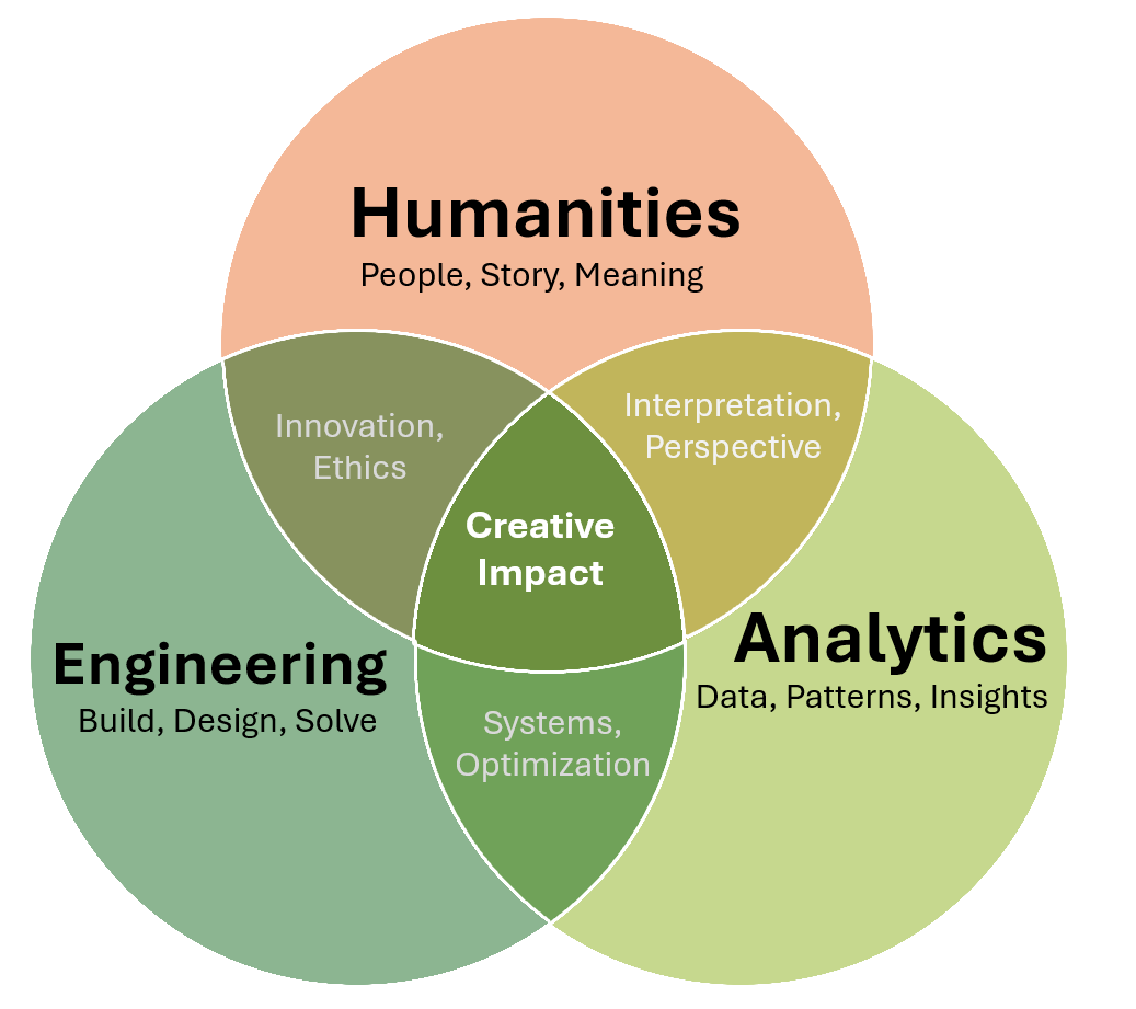
Engineering and analytics give us the tools to build and understand complex systems, from energy grids to economic models. But the humanities help us ask the right questions. They remind us that technology doesn’t exist in a vacuum; it shapes and is shaped by people, culture, and history. To truly innovate, we need both—the precision of data and the depth of human insight.
Data can reveal social truths that impacts every individual, engineered solutions can be more effective when they consider human behavior, and storytelling and history can influence innovation. The world is built on connections between people, ideas, and disciplines. For me, the best way to make an impact is by embracing that interconnectedness, by considering what happens when we bring these fields together. This consideration fuels my curiosity, my work, and my passion for exploring the bigger picture.
Engineering
Engineering is the art of creation and problem-solving. It takes the world’s biggest challenges and transforms them into opportunities for innovation. At its heart, it’s about understanding systems and making them more efficient, reliable, and sustainable, all the while blending logic, creativity, and vision to shape the world around us. It’s a field that thrives on curiosity, asking not just how things work, but how they could work better. Whether it’s designing smarter cities, optimizing renewable energy, or advancing technology, engineering is about building what comes next.
Systems Thinking
Engineers solve problems by designing systems. Whether it’s infrastructure, software, energy grids, or manufacturing, real-world engineering challenges aren’t isolated. They exist within immensely complex, interconnected systems, where one change can influence everything else.
Systems thinking is a way of making sense of this complexity. Instead of just focusing on individual components, engineers look at how things interact, how information flows, and how small adjustments ripple through the entire system. Instead of focusing on individual parts, it’s about stepping back and looking at the bigger picture. Engineers ask:
- What are the key parts of this system?
- How do they influence each other?
- What happens if something changes?
- How can we optimize for efficiency, stability, or adaptability?
Most engineering systems can be broken down into:
| Component | Definition | Example |
|---|---|---|
| System | The entire structure with all its interconnected parts | Electrical grid |
| Subsystem | A functional unit within the larger system | Power generation, transmission, distribution |
| Unit Type | A specific element within a subsystem | Turbine, transformer, solar panel |
| Operations | The processes that keep the system running | Energy flow, load balancing, grid frequency regulation |
Understanding systems isn’t just about making things more efficient; it’s about making them work better as a whole, long-term. Without a systems mindset, solutions can be short-sighted, solving one issue while creating several new ones. Systems thinking prevents this by keeping the bigger picture in focus. In an increasingly complex world, the ability to step back, recognize patterns, and optimize for the bigger picture is what separates quick fixes from long-lasting solutions.
Energy Systems
Energy is everywhere. It moves our bodies, fuels our machines, and powers our cities. But energy itself doesn’t appear or disappear—it transforms. This is the foundation of thermodynamics, the study of how energy moves and changes forms.
At its core is the conservation of energy, which states that energy cannot be created or destroyed, only converted. Whether in a boiling pot of water, a moving car, or a power plant, the same principle applies:
\[ \Delta E = Q - W \] Expanding for all forms of energy:
\[ \Delta U + \Delta KE + \Delta PE = Q - W + m \left( \frac{P}{\rho} \right) \]
Where:
- \(U\) = Internal energy (heat stored inside an object)
- \(KE\) = Kinetic energy (energy from movement)
- \(PE\) = Potential energy (energy due to position)
- \(Q\) = Heat transfer (energy added or removed)
- \(W\) = Work done (energy used to move something)
- \(m\) = Mass (amount of matter in the system)
- \(P\), \(\rho\) = Fluid pressure and density (energy in flowing fluids)
These equation may look merely theoretical, but they are the blueprint for modern civilization. By understanding how energy moves, engineers have designed systems that harness it efficiently, from the simplest engines to the most advanced power grids. In fact, humans have used energy transformation to our advantage for thousands of years:
- Fire (Chemical → Thermal Energy) – Early civilizations burned wood to cook, stay warm, and forge metal.
- Steam Engines (Chemical → Thermal → Mechanical Energy) – In the 1700s, steam engines transformed heat from burning coal into movement, powering trains and industry.
- Power Plants (Chemical → Thermal → Mechanical → Electrical Energy) – The industrial revolution introduced power plants, scaling up energy conversion to produce electricity for entire cities. Common fuels used include coal, natural gas, and uranium.
- Renewables (Wind, Solar, Hydro) – Today, we’re transitioning to energy sources that convert natural forces directly into electricity—wind turbines (Kinetic → Electrical), solar photovoltaics (Light → Electrical), and hydroelectric dams (Mechanical → Electrical Energy).
Energy is the foundation of civilization. From early fire to modern power grids, the ability to transform and distribute it efficiently has shaped history. As technology advances, the way we generate and manage energy will define the future. Improving efficiency, integrating renewables, and designing smarter grids are challenges that will impact sustainability, industry, and daily life, making energy an important and exciting fields to explore.
Electrical Grid
According to the National Academy of Engineering, the number one greatest engineering achievement of the 20th century is electrification. It has enabled modern civilization, from lighting cities to powering industries, transforming nearly every aspect of daily life. Yet, over a century after its invention, the grid still operates on a rigid, century-old framework: power plants generate electricity, transmission lines carry it vast distances, and distribution networks deliver it to homes and businesses. This system has worked remarkably well—but it was built for a different era, one without widespread renewable energy or real-time analytics.
The challenge today is not only to generate enough electricity, but distributing it efficiently in a rapidly changing world. Renewable energy sources like wind and solar introduce variability, requiring new approaches to maintaining a stable power supply. Climate change adds further urgency, demanding that we rethink how electricity is generated, stored, and delivered.
At its core, the grid is a network of interconnected subsystems, each with a crucial role:
- Power Generation – Energy is produced through coal, natural gas, nuclear, hydro, wind, and solar power.
- Transmission – High-voltage lines move electricity efficiently across long distances.
- Distribution – Local networks step down the voltage and deliver power to homes and businesses.
For over a century, these components have worked together to provide reliable electricity. But integrating intermittent renewables disrupts this balance, introducing complexities that traditional grid models weren’t designed for. The grid must match electricity supply with demand at every moment, but not all power sources operate the same way:
- Baseline power – Consistently running power plants, such as nuclear and coal, provide a steady supply of electricity.
- Peaker plants – Gas-powered plants can ramp up quickly during high demand but are expensive and inefficient to run frequently.
- Intermittent renewables– Solar and wind produce energy when nature allows, which doesn’t always align with demand.
Historically, baseline plants handled the majority of energy needs, while peaker plants filled in gaps during peak hours. But as renewables become more common, they disrupt this balance. Without better energy storage or grid flexibility, excess solar energy at noon can go to waste, while evening peaks still rely on fossil fuels.
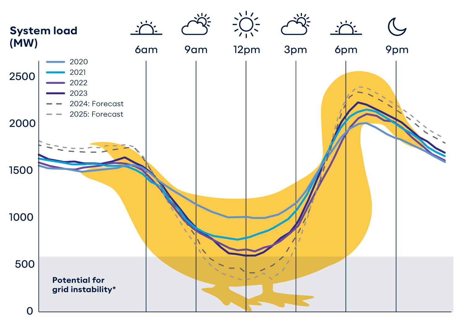
Renewable energy generation can lead to overproduction when demand is low and shortages when demand is high. To manage this, grid operators must either curtail excess energy (wasting it) or store it for later use (which is currently limited). The goal is to flatten the duck curve by spreading out electricity demand and improving storage solutions. In other words, we need to make the grid a little less duck-shaped—because while ducks are great in ponds, they make for a pretty unstable energy system.
A quick note on supply and demand. Every year, our demand for electricity increases (i.e. more data centers, more electric vehicles, more air conditioning), but power generation remains relatively constant. This may seem counterintuitive, but it’s largely due to energy efficiency improvements. LED lighting, smarter appliances, and improved industrial processes allow us to do more with the same amount of energy. However, even with these gains, the shift to electrified transportation and digital infrastructure means we must rethink how we scale energy production.
Tomorrow’s grid must be smarter, more flexible, and data-driven. Engineers and analysts are developing solutions such as:
- Battery storage – Capturing excess renewable energy for later use.
- Decentralized microgrids – Local energy networks that improve resilience.
- Real-time analytics – Predicting demand fluctuations and optimizing power flow.
- Automated grid management – AI-driven decision-making for efficiency.
The grid may look only like infraastructure, but it is a complex dynamic system that shapes economies and societies. Transforming the grid requires balancing reliability, affordability, and sustainability. Simulating future grid scenarios with data analytics will help ensure a system that works for everyone and defines the future.
Analytics
Analytics is about making sense of the world through patterns, predictions, and decisions. It’s a way to represent reality—but no model is a perfect reflection of realitye. As statistician George Box famously put it, “All models are wrong, but some are useful.” Models simplify complex systems, stripping away details to highlight key relationships. They may not capture every nuance to be the truth, but they provide structured approximations that help us understand complexity.
Modeling is often seen as a science, but it’s just as much an art. It requires judgment, interpretation, and creativity in defining assumptions, selecting variables, and refining results. Data alone doesn’t tell the full story; the real skill lies in knowing what to model, how to structure it, and where its limitations lie. Whether analyzing trends, forecasting outcomes, or optimizing decisions, analytics builds useful representations of reality—ones that allow us to think critically, make informed decisions, and continuously refine our understanding.
Exploratory Data Analysis
Before building any models, data must be explored, cleaned, and understood. Exploratory Data Analysis (EDA) is the process of investigating raw data, identifying patterns, and preparing it for meaningful analysis. The reality is that the majority of data science is not about advanced modeling at all; rather, it’s about making sense of messy, real-world data.
As John Tukey famously said, “Embrace your data, not your models.” A model is only as good as the data feeding it. Without a deep understanding of the data itself, even the most sophisticated model will be misleading at best and completely wrong at worst.
In a perfect world, data would be pristine: consistent, complete, and ready for analysis. Unfortunately, real-world data rarely looks like that. Instead, it comes from multiple sources, gets entered manually, is often missing key details, and sometimes outright wrong. Consider a few real-life challenges:
- Inconsistent Formatting – A name might appear as
"J. DOE","JOHN DOE","john doe", or"John A. Doe", making identity matching difficult. - Entry Errors – A missing decimal could turn
$100.00into$10,000.00, creating a major outlier. - Conflicting Date Formats –
"1 January 1970"and"01/01/1970"are the same date but require standardization. - Records Discrepancies – A hospital’s patient records may vary depending on how different doctors enter information.
- Survey Gaps – Respondents may skip questions, leading to missing values.
- Sensor Malfunctions – Weather stations sometimes record impossible temperatures due to hardware failures.
Messy data is everywhere, but it is where data science begins. A robust, well-documented, and reproducible EDA process is the foundation of reliable analysis. Without it, conclusions are flawed, models are unreliable, and insights become meaningless. Understanding what’s missing, what’s misleading, and what might introduce bias is critical before drawing any conclusions.
One of the quickest ways to summarize and explore data is through pivot tables. They allow analysts to dynamically slice and dice information across different categories, compute aggregates (like sums, averages, and counts), and uncover hidden trends.
Below is an interactive pivot table using rpivotTable that breaks down CO₂ emissions by vehicle type. Try selecting different attributes like MPG or weight to see how they relate.
Numbers in a table can provide insight, but visualization is an intuitiive way to explore data. Charts and graphs help reveal trends, outliers, and relationships in ways that raw numbers can’t. A few common techniques include boxplots, histograms, and scatterplots.
The boxplot below provides a clear visualization of the same CO₂ emission data from the pivot table.
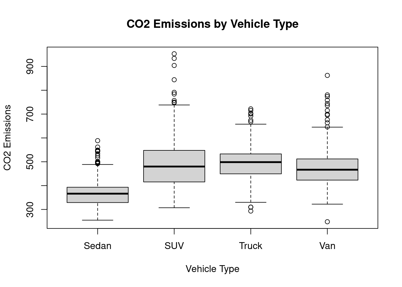
Intuitively, the result makes sense: the bigger the vehicle, the higher the emissions. But how strong is this relationship? Is weight the only factor? To understand this better, we need to examine correlation.
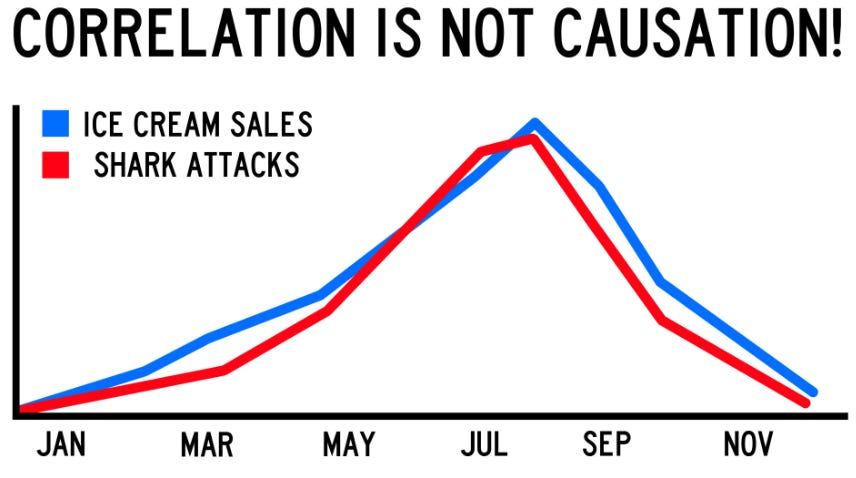
One of the biggest pitfalls in analysis is mistaking correlation for causation. Correlation does not result in causation; just because two variables move together doesn’t mean one is causing the other. Without deeper investigation, data can tell a misleading story that might seem logical at first but falls apart with further scrutiny. The classic example of ice cream sales and shark attacks illustrates this perfectly.
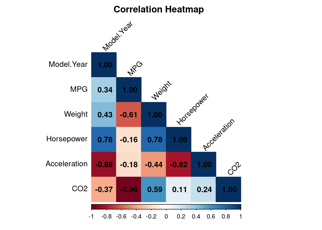
Below is a correlation heatmap of our dataset, revealing the key relationships between vehicle attributes. CO₂ emissions strongly correlate with MPG, model year, and weight. This intuitively makes sense; fuel-efficient cars emit less CO₂, newer models tend to be cleaner, and heavier vehicles produce more emissions.
Remember, EDA is not optional—it is the most important step in any data analysis. Without it, models are built on assumptions rather than reality. By thoroughly exploring data, we can identify patterns, question biases, and refine our approach before jumping to conclusions. A great model can’t fix bad data, but great EDA can prevent bad models.
Types of Models
The table below breaks down different modeling approaches, from supervised and unsupervised learning to time-series analysis and probability-based methods. These categories help define how data is used, whether it’s predicting an outcome, grouping similar observations, or analyzing uncertainty.
| Category | Models & Techniques | Purpose |
|---|---|---|
| Supervised Learning | Classificaiton (SVM, KNN), Regression (Linear, Logistic, Advanced), Decision Trees (CART, Random Forests), Neural Networks (Deep Learning) | Uses labeled data to predict outcomes. |
| Unsupervised Learning | Clustering (k-Means, DBSCAN), Dimensionality Reduction (PCA) | Finds patterns in unlabeled data. |
| Time-Series Models | Forecasting (ARIMA, GARCH), Trend Analysis (Exponential Smoothing), Change Detection (CUSUM) | Analyzes temporal dependencies for trend prediction. |
| Probability-Based Models | Distribution Fitting, A/B Testing, Markov Chains, Bayesian Statistics, Simulation | Models uncertainty and probabilistic relationships. |
This may seem like an abstract technical concepts, but models like these actually help us make sense of the world. In a way, they’re not so different from how we think; after all, our brains function like neural networks, constantly learning from past experiences (our “training data”, if you will) and adjusting based on new information. We don’t need massive datasets or code to do it, but the process is familiar: we take in patterns, form expectations, and refine our judgment.
Modeling Process
The second table below walks through the full data modeling pipeline, from preparing raw data to engineering meaningful features, applying descriptive, predictive, or prescriptive models, and finally ensuring the model is validated and deployable. Each step plays a role in making data-driven decisions more accurate, reliable, and actionable.
| Stage | Key Concepts | Purpose |
|---|---|---|
| Pre-Modeling (Data Preparation) | Outlier Detection, Data Cleaning, Transformations, Scaling, Imputation | Ensures clean, high-quality data before modeling. |
| Feature Engineering | Variable Selection, Principal Component Analysis (PCA) | Reduces dimensionality and improves model performance. |
| Descriptive Models | Summary Statistics, Data Visualization, Clustering | Identifies patterns, trends, and structure in data. |
| Predictive Models | Supervised Learning, Time-Series Forecasting | Finds hidden relationships and forecasts future trends. |
| Prescriptive Models | Optimization, Simulation, Game Theory, Reinforcement Learning | Recommends actions to maximize desired outcomes. |
| Post-Modeling (Deployment) | Cross-validation, Model Evaluation, Bias Detection, Interpretability | Ensures reliability, fairness, and usability of models. |
In many ways, this process mirrors how we reason and navigate the world. We:
- Gather information first: just like pre-modeling data preparation.
- Find patterns: similar to descriptive models identifying trends.
- Make predictions: drawing from past experiences, much like predictive models.
- Make decisions: choosing the best action, just like prescriptive models.
We start by gathering information (pre-modeling), focus on what matters (feature engineering), recognize patterns (descriptive models), anticipate outcomes (predictive models), and, when possible, make decisions to optimize results (prescriptive models). Then we deploy our model by communicating to others—though whether that “model” is fair, accurate, or completely overfitted to our own biases is a whole other discussion (and probably a debate waiting to happen).
Understanding this structure helps clarify when and why different techniques are used. Not every project needs all three modeling types (descriptive, predictive, and prescriptive), but seeing how they interact allows for better problem-solving and decision-making.
And just like AI, we’re constantly learning, adapting, refining, and making decisions based on experience. Whether we’re analyzing data, forecasting the future, or optimizing outcomes, these models are shaping technology and reflect how we think, reason, and make sense of the world.
Regression
Regression is one of the most fundamental and widely used tools in analytics, and for good reason. At its core, regression helps us quantify relationships between variables, making it a go-to method in research, economics, engineering, and even everyday decision-making. It’s also incredibly intuitive—we recognize patterns constantly in our daily lives. For example, we know that more study hours tend to result in better grades, increased exercise often leads to improved health, and a car’s fuel efficiency correlates with its CO₂ emissions. Regression formalizes these observations into a mathematical framework to predict future outcomes.
Despite its power, regression isn’t infallible. It relies on key assumptions:
| Assumption | Definition | Diagnostic Tool | Resolution |
|---|---|---|---|
| Linearity | The relationship between the independent and dependent variables should be linear. | Scatter plots, Residual vs. Fitted plots | Apply logarithmic, square root, or polynomial transformations. |
| Homoscedasticity | The variance of residuals should remain constant across all levels of the independent variable(s). | Residual vs. Fitted plot | Use Box-Cox transformation (on response variable), log transformation, or weighted least squares. |
| Normality of Residuals | The residuals should be normally distributed for valid hypothesis testing. | Q-Q Plots, Histograms | Apply transformations (log, Box-Cox) to the dependent variable. Only evaluate normality using residuals, not the response variable. |
| Independence of Errors | Observations should not be correlated over time (no autocorrelation). | Durbin-Watson test, Residual vs. Time plot | If data is from a randomized trial, independence is likely established. If from observational studies, check for uncorrelated errors rather than independent errors. |
| No Multicollinearity | Independent variables should not be highly correlated with each other. | Variance Inflation Factor (VIF), Correlation matrix | Remove/combine highly correlated variables, use PCA, or use lasso, ridge, or elastic net regression. |
| No Outliers | Outliers and high-leverage points should not disproportionately impact the regression model. | Cook’s Distance, Leverage plots, Box plots | Correct or remove. |
| Adequate Sample Size | Ensures sufficient observations per predictor variable to avoid overfitting. | Rule of thumb: at least 10-15 observations per predictor variable | Increase sample size if necessary to ensure stable coefficient estimates. |
| Additivity | Interaction effects should be accounted for when necessary. | Test for significant interaction terms. | Include interaction terms in the model if needed. |
Violating regression assumptions can distort results and lead to unreliable models. This is why diagnostic tools are essential in EDA to assess whether a model or its data is valid before blindly trusting it.
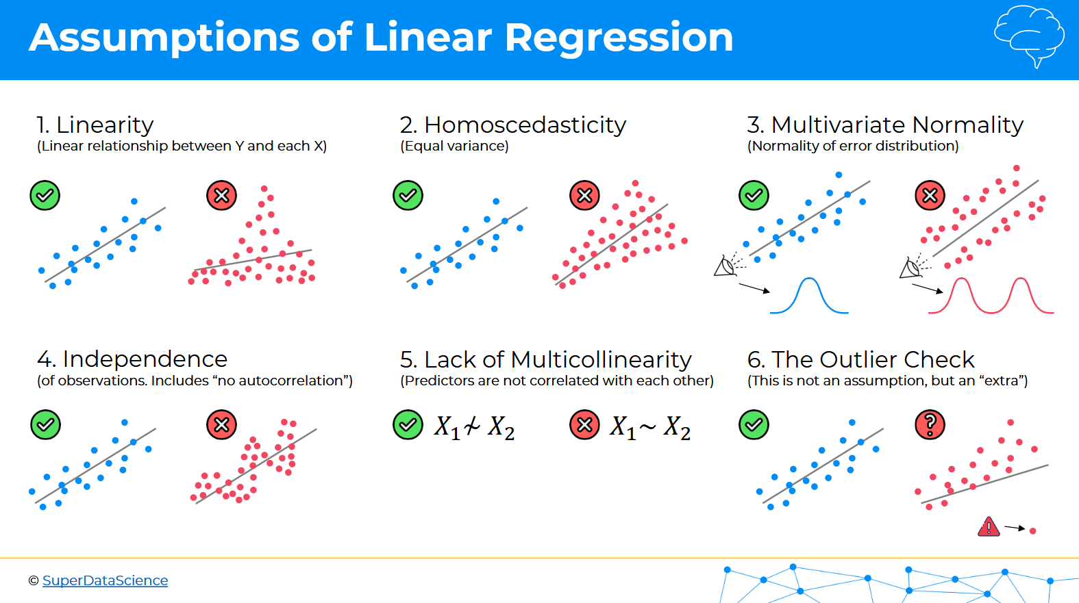
1) Linearity ensures that the relationship between variables follows a straight-line pattern; if a curved trend appears, consider transforming the variables.
2) Homoscedasticity assumes that residuals have constant variance. When this is violated (as seen in the right image with a funnel shape), a non-linear transformation (linear-linear, linear-log, log-linear, log-log) can help.
3) Multivariate normality requires residuals to be normally distributed for reliable statistical inference. If errors are skewed, try removing extreme outliers.
4) Independence assumes that observations aren’t correlated over time (no autocorrelation). For time-series data, this often means incorporating lag terms or using time-series models like ARIMA. For non-time series data, look for clustered or grouped data to restructure, where observations within the same group are correlated.
5) Multicollinearity occurs when predictors are highly correlated, which can distort coefficient estimates. This can be fixed by removing redundant variables, PCA, or applying lasso, ridge, or elastic net regression.
6) While outliers aren’t strictly an assumption, they can heavily influence regression results; visualization tools like boxplots and influence diagnostics can help detect them.
At its simplest, regression estimates the relationship between an independent variable (predictor) and a dependent variable (outcome). The most common type is linear regression, which assumes a straight-line relationship:
\(Y = \beta_0 + \beta_1 X + \varepsilon\)
Where:
- \(Y\) = dependent variable (the response we want to predict)
- \(X\) = independent variable (the predictor)
- \(\beta_0\) = intercept (the baseline value of \(Y\) when \(X\) is zero)
- \(\beta_1\) = slope (how much \(Y\) changes for each unit increase in \(X\))
- \(\varepsilon\) = error term (representing variability not explained by the model)
Regression models draw a best-fit line through data points, aiming to get as close as possible to the actual values while minimizing the difference between predictions and reality. However, no model is perfect—there will always be some error. Residuals represent the gap between what a model predicts and what actually happens. To measure how well a model fits the data, regression minimizes the sum of squared residuals—meaning it finds the line that keeps errors as small as possible while avoiding overcomplicating the model. Squaring the residuals ensures that large mistakes are penalized more, leading to a more reliable and stable model.
In many real-world scenarios, a single predictor isn’t enough to explain an outcome. This is where multiple regression comes into play. Instead of modeling one independent variable (\(X\)), multiple regression incorporates multiple predictors (\(X_n\)):
\(Y = \beta_0 + \beta_1 X_1 + \beta_2 X_2 + ... + \beta_n X_n + \varepsilon\)
Sometimes, categorical variables (like “car type” or “region”) need to be included in a model. Since regression requires numerical inputs, we introduce dummy variables (indicator variables) to represent categories. For example, a dataset with “Sedan” and “Truck” cars could use a dummy variable where Sedan = 0 and Truck = 1. This allows regression models to incorporate qualitative factors and estimate their impact on the dependent variable.
Beyond individual predictors, variables can interact with each other in meaningful ways. Interaction terms allow us to capture these effects. For instance, the effect of weight on CO₂ emissions might differ depending on whether a car is a sedan or truck. Instead of assuming weight has the same effect across all cars, an interaction term (i.e. Weight × Type) would account for this difference. Interaction terms can reveal complex relationships and reduce multi-collinearity.
Other specialized forms of regression include:
- Logistic Regression: Used when the outcome is categorical (i.e. Yes/No, On/Off, Red/Blue/Yellow).
- Polynomial Regression: Captures non-linear relationships by fitting curves instead of straight lines.
- Ridge, Lasso, and Elastic Net Regression: Address overfitting and improve predictive power by applying penalties to model complexity.
Now, let’s return to our CO₂ emissions dataset. Intuitively, we expect larger vehicles to emit more CO₂, but how strong is that relationship? Using regression, we can quantify how much an increase in weight or horsepower influences emissions.
We define a linear regression model where CO₂ emissions (\(Y\)) are predicted based on multiple factors (\(X_n\)):
\(CO₂ = \beta_0 + \beta_1 \times Weight + \beta_2 \times MPG + \beta_3 \times Model.Year + \varepsilon\)
Now we’re ready to run the regression.
model <- lm(CO2 ~ MPG + Weight + Model.Year, data = data)
summary(model)
Call:
lm(formula = CO2 ~ MPG + Weight + Model.Year, data = data)

Residuals:
    Min      1Q  Median      3Q     Max
-39.564 -14.362  -6.149   6.326 254.785

Coefficients:
              Estimate Std. Error t value Pr(>|t|)
(Intercept)  3.875e+03  1.952e+02   19.86   <2e-16 ***
MPG         -1.629e+01  3.359e-01  -48.49   <2e-16 ***
Weight       2.850e-02  2.084e-03   13.68   <2e-16 ***
Model.Year  -1.600e+00  1.040e-01  -15.39   <2e-16 ***
---
Signif. codes:  0 '***' 0.001 '**' 0.01 '*' 0.05 '.' 0.1 ' ' 1

Residual standard error: 25.17 on 1699 degrees of freedom
Multiple R-squared:  0.9296,    Adjusted R-squared:  0.9295
F-statistic:  7482 on 3 and 1699 DF,  p-value: < 2.2e-16
The regression results provide insights into the relationship between CO₂ emissions (g/mile) and three predictors: MPG (fuel efficiency), vehicle weight, and model year.
- The negative coefficient for MPG (-1.629) indicates that for each additional mile per gallon a vehicle achieves, CO₂ emissions decrease by approximately 1.63 g/mile, which aligns with expectations—more fuel-efficient cars produce less CO₂.
- The positive coefficient for weight (2.85) suggests that for every additional unit of vehicle weight, CO₂ emissions increase by about 2.85 g/mile, reinforcing the idea that heavier vehicles require more energy to move.
- The model year coefficient (-1.60) suggests that for each newer model year, CO₂ emissions decrease by 1.6 g/mile, likely due to advancements in fuel efficiency and emissions regulations over time.
- The intercept (3875 g/mile) represents the theoretical CO₂ emissions when all predictor variables are zero, though this isn’t a meaningful real-world scenario.
- All predictors are highly statistically significant (p-values < 2e-16), indicating strong evidence that these factors influence emissions.
- The R-squared value (0.9296) suggests that the model explains about 92.96% of the variation in CO₂ emissions, meaning the chosen predictors provide a strong fit to the data.
- The F-statistic (7482, p < 2.2e-16) confirms that the overall model is highly significant.
In summary, this model confirms the expected trends—higher MPG and newer model years reduce emissions, while heavier vehicles contribute to increased CO₂ output. All done, right? Not quite. We did not look to see if the dataset violated the assumptions of regression. Let’s run a couple of visual diagnostics.
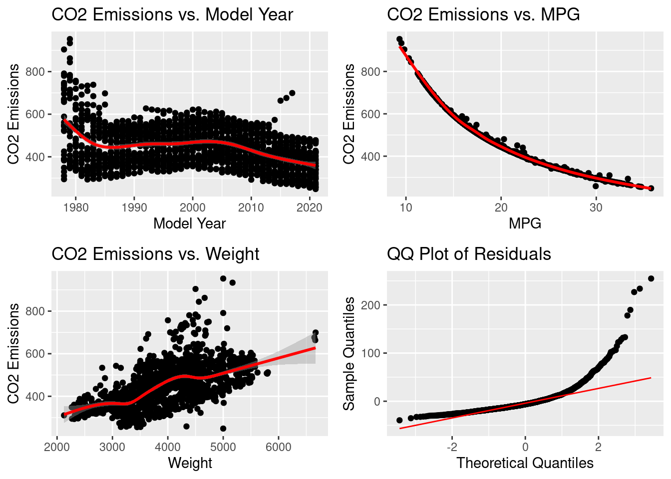
Uh oh, looks like our regression assumptions aren’t holding up well. The CO₂ vs. Model Year plot shows a nonlinear trend, violating the assumption of linearity. The CO₂ vs. MPG plot has a clear nonlinear pattern, suggesting a transformation (i.e. log transformation) could help linearize the relationship. The CO₂ vs. Weight plot shows increasing variance in residuals, indicating heteroscedasticity. The QQ plot of residuals reveals a heavy-tailed distribution, violating normality of residuals. Ideally, residuals should be normally distributed, homoscedastic, and independent, with a linear relationship between predictors and the outcome. These diagnostics helped us discover that the data by itself is not ready for modeling since it violates the assumptions of regression. To fix these issues, we can explore techniques shown in the table above, and also apply dummy variables and interaction terms.
Humanities
Now on to my favorite subject! Though my career is in engineering and analytics, I spend much of my free time reading and thinking about history, philosophy, anthropology, sociology, and psychology. Science and data model how things work, but the humanities ask why they matter, exploring culture, morality, identity, and power. They reveal the patterns in history, thought, and society, much like an engineer studies interconnected systems or an analyst uncovers trends in data. The humanities challenge us to think bigger picture, question assumptions, and engage with complexity, providing the context to what it means to be human.
Anthropology
How did we get here? Homo sapiens have existed for nearly 300,000 years, yet the world we live in today—our cities, economies, technologies—has emerged only in a fraction of that time. For most of human history, we were hunter-gatherers, navigating the world in small, mobile groups. Civilization as we know it is a recent development, built on a series of transformative shifts that reshaped how we think, interact, and organize society. Anthropology examines these changes, uncovering patterns in human culture, behavior, and adaptation while posing a key question:
How does our evolutionary past still shape us today?
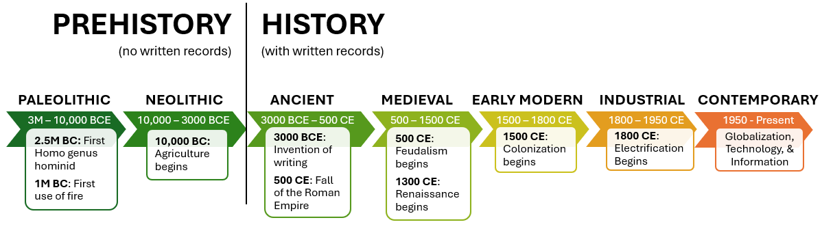
For most of human history, written records didn’t exist. This period is known as prehistory and was defined by survival adaptation and traditions passed down through generations. Early hominids like Neanderthals and Denisovans coexisted with Homo sapiens, but what set Homo sapiens apart was cooperation, imagination, and adaptability—traits that ultimately made them the only surviving species of the Homo genus.
The Cognitive Revolution (~70,000 years ago) was a key moment in this process, marking the emergence of abstract thought, symbolic language, and cultural belief systems, which laid the foundation for everything that followed.
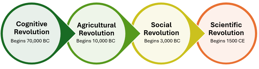
Each major shift in human history transformed how we lived:
- Cognitive Revolution (~70,000 years ago): Expanded our ability to reason, plan, and organize in large groups.
- Agricultural Revolution (~10,000 years ago): Allowed humans to settle, grow food, and establish permanent communities, leading to population growth but also introducing social hierarchies, property disputes, and disease.
- Social Revolution (~5,000 years ago): Formalized social structures through laws, religion, and economies, shaping governance and collective identity.
- Scientific Revolution (~500 years ago): Fueled rapid technological advancements, transforming industries, global power structures, and our relationship with the environment.
These transitions didn’t happen overnight. No one at the time could have foreseen their impact, as each phase unfolded gradually over thousands of years, with both progress and unintended consequences.
To truly grasp the scale of these changes, explore the interactive treemap below. It visually represents how much time each period spans, offering a striking perspective on just how recent civilization, as we know it, really is.
So, why does this matter? Because our biological evolution hasn’t kept pace with the world we’ve created. The human brain evolved to function in small, close-knit communities, prioritizing immediate rewards and quick decision-making that were advantageous for survival. While these instinctual processes still influence behavior, the brain has also developed complex networks that support long-term planning, abstract reasoning, and technological innovation. These cognitive abilities allowed us to build civilizations, develop science, and expand our collective knowledge.
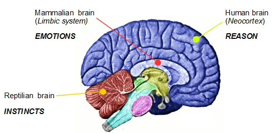
The tension between these two sides of the brain drives much of human behavior today. We are wired for rapid, emotionally charged responses driven by deep-seated survival mechanisms, yet we also engage in complex reasoning and problem-solving. This tension explains so much about human behavior: why we struggle with long-term decision-making, why fear and tribalism still drive much of our politics, and why expoential technologyical advancement can feel overwhelming to a species adapted for gradual change. No one is immune to the evolutionary forces that shaped us.
Understanding where we came from helps us make sense of where we are now. Our instincts were shaped for a prehistoric world, yet we navigate an modern world of artificial intelligence, mass information, and rapid globalization. It’s as if we’re running on an outdated operating system, trying to process technological advancements that outpace our current cognitive evolution.
It took us tens of thousands of years to develop abstract thought, after all. Will we one day see another Cognitive Revolution, one that can handle today’s information input? Or is technology evolving too fast for us to keep up? If history has shown us anything, it’s that humans are capable of extraordinary transformation. The real question is: where do we go from here?
History & Religion
History is often divided into broad periods based on technological advancements, societal organization, and dominant ideologies. The general progression follows:
- Stone Age → Ancient → Medieval → Modern
In historical sequence:
- Prehistory → Ancient Greece & the Roman Empire → Feudalism & Religion (Dark Ages) → Enlightenment → Globalization & Science
These transitions were influenced by factors such as Marx’s theory of history and dialectical materialism, which frames history as a struggle between economic classes, and political evolution from tribes → kingdoms → empires.
The table below outlines major historical ages, their defining characteristics, and key events that shaped human civilization.
| Age | Name of Era | Year Period | # of Years | Main Event | Details of Events |
|---|---|---|---|---|---|
| Stone | Paleolithic | 3,000,000 - 10,000 BCE | 2,990,000 | Homo sapien evolution and the Ice Age | Use of stone tools, development of language, early art |
| Stone | Mesolithic | 10,000 - 8,000 BCE | 2,000 | Transition to farming | Domestication of animals, microlithic tools, early settlements |
| Stone | Neolithic | 8,000 - 3,000 BCE | 5,000 | Agricultural revolution | Permanent settlements, pottery, weaving, advanced tools |
| Ancient | Bronze Age | 3,000 - 1,200 BCE | 1,800 | Writing and structured civilization | Development of writing systems, organized civilization, trade networks |
| Ancient | Iron Age | 1,200 - 500 BCE | 700 | Rise of empires | Widespread iron use, territorial expansion, centralized rule |
| Ancient | Classical Antiquity | 500 BCE - 500 CE | 1,000 | Expansion and political structures | Urbanization, philosophy, governance, large-scale conflicts |
| Medieval | Early Middle Ages | 500 - 1000 CE | 500 | Decentralization and rise of feudalism | Local rule, decline of urban centers, self-sufficient economies |
| Medieval | High Middle Ages | 1000 - 1300 CE | 300 | Crusades and scholasticism | Religious control over society, universities, increased trade |
| Medieval | Late Middle Ages | 1300 - 1500 CE | 200 | Crisis and early Enlightenment thought | Black Death, political unrest, scientific exploration, early Enlightenment |
| Modern | Early Modern Period | 1500 - 1800 CE | 300 | Renaissance and colonization | Global exploration, reformation, scientific advancements |
| Modern | Industrial Age | 1800 - 1950 CE | 150 | Industrialization and world wars | Factories, steam power, electrification, world wars |
| Modern | Contemporary Era | 1950 - Present | 70 | Digital and globalized information | Computers, internet, space exploration, globalization |
Each period represents shifts in economic structures, governance, and technological innovations. The transition from hunter-gatherer societies in the Paleolithic Age to agrarian communities in the Neolithic Age set the foundation for the rise of civilizations. The Bronze and Iron Ages introduced writing, trade networks, and structured governance, leading to Classical Antiquity, which saw the emergence of philosophy, law, and empire-building.
The Medieval Period marked decentralization following the collapse of the Roman Empire, with feudalism dominating Europe. The Renaissance and Early Modern Period spurred exploration, scientific thought, and global interactions, leading into the Industrial Age, where mechanization and world wars reshaped human progress. Finally, the Contemporary Era is defined by digital globalization and rapid technological advancements.
While broad historical ages provide structure, civilizations themselves had distinct trajectories. Some expanded through conquest, others thrived through trade, and many fell due to internal decline or external pressures. The chart below visualizes major civilizations across different regions and their timelines.
From the ancient cities of Mesopotamia and Egypt to the global empires of modern times, each civilization adapted to its environment and left lasting cultural, political, and technological legacies. The decline of empires often coincided with shifts in governance, economic instability, or military conflicts.
Religion has played a fundamental role in shaping human history, often driving social cohesion, political authority, and cultural identity. Many empires justified their rule through divine mandate, while religious movements have both unified and fractured societies.
The timeline below illustrates the emergence of major world religions and their regions of origin.
From polytheistic traditions in ancient civilizations to the rise of monotheistic faiths and their global influence, religion has shaped governance, philosophy, and societal norms. The dominance of certain religious traditions in specific eras often coincided with the rise of corresponding empires.
Looking at long-term trends, several patterns emerge:
The Dark Ages and Intellectual Revival: Following the collapse of the Roman Empire, Europe entered a period of feudal fragmentation. However, the Islamic Golden Age preserved and expanded knowledge, influencing the later European Renaissance.
Eurocentric Historical Narratives: While dominant global narratives often focus on Europe’s progression, civilizations in Asia, Africa, and the Americas played equally vital roles in shaping human history.
Cyclical Patterns: Some historians suggest that history follows cyclical patterns, such as the Strauss-Howe generational theory, which proposes societal shifts occurring approximately every 250 years.
Understanding history through these frameworks allows us to recognize past patterns, appreciate diverse contributions, and anticipate potential future shifts.
to include: - rites, rituals, community -> very human - more high lvl look at religion origins
Philosophy
Under Construction
- Socrates
- Plato
- Aristotle (bring up catharsis; more on this in sociology)
- hedonism vs. cynic vs. stoic
- Descartes
Sociology
Under Construction
- the medium is the message
- the culture industry
- reclaiming conversations
- bowling alone
- amusing ourselves to death
Psychology
Under Construction
- history: freud, jung, Edward Bernays, etc
- personal trauma
- cultural trauma (advertising, hustle culture, honor)
- personality disorders
- rational vs emotional mind vs wise mind (DBT)
- different therapy modalities